NicheDECODE Tutorial

Overview

NicheDECODE estimates niche-level spatial architecture abundance from tissue-level omics data. The repository contains reusable model code, data-processing utilities, experiment notebooks, saved model checkpoints, and example prediction outputs.

1. Build pseudo-tissue data Generate spatial sliding-window and random mixed-cell pseudo-bulk samples from annotated spatial single-cell data.

2. Add spatial features Merge expression profiles with gene-wise spatial variability features and graph-derived gene relationships.

3. Train NicheDECODE Fit the encoder, GCN feature gate, and predictor, then export predicted niche proportions and evaluation metrics.

Quick start

Clone the repository and create the conda environment from the provided specification.

git clone https://github.com/forceworker/NicheDECODE_main.git
cd NicheDECODE_main
conda env create --name nichedecode -f environment.yml
conda activate nichedecode

Launch Jupyter Lab from the repository root so that imports such as from data.dataProcess import * and from model.nicheDeconv import * resolve correctly.

jupyter lab

The implementation uses CUDA tensors in the model workflow. A CUDA-enabled PyTorch environment is recommended for reproducing the training notebooks without code changes.

Data and files

The repository points to public Zenodo archives for the full data and notebook records. Download the required data files before running the data-processing notebooks.

Resource	Location	Purpose
Data archive	10.5281/zenodo.18856556	Input data used for the NicheDECODE examples.
Notebook records	Zenodo record 18857669	Jupyter records for the experiments described in the work.
Example notebooks	`data/human_nsclc/`, `data/CODEX/`, `exp/human_nsclc/`, `exp/CODEX/`	Data construction, model training, prediction, and evaluation workflows.
Saved checkpoints	`save_models/human_nsclc/best_model.pt`, `save_models/CODEX/best_model.pt`	Pretrained checkpoints used by the example prediction notebooks when present.
Example outputs	`res/human_nsclc/`, `res/CODEX/`	Predicted niche proportions and corresponding ground-truth proportions.

Prepare pseudo-tissue data

Use the data-processing notebooks first. They construct training and test pseudo-tissue samples and save normalized files consumed by the model notebooks.

Human NSCLC example

cd data/human_nsclc
jupyter lab data_process.ipynb

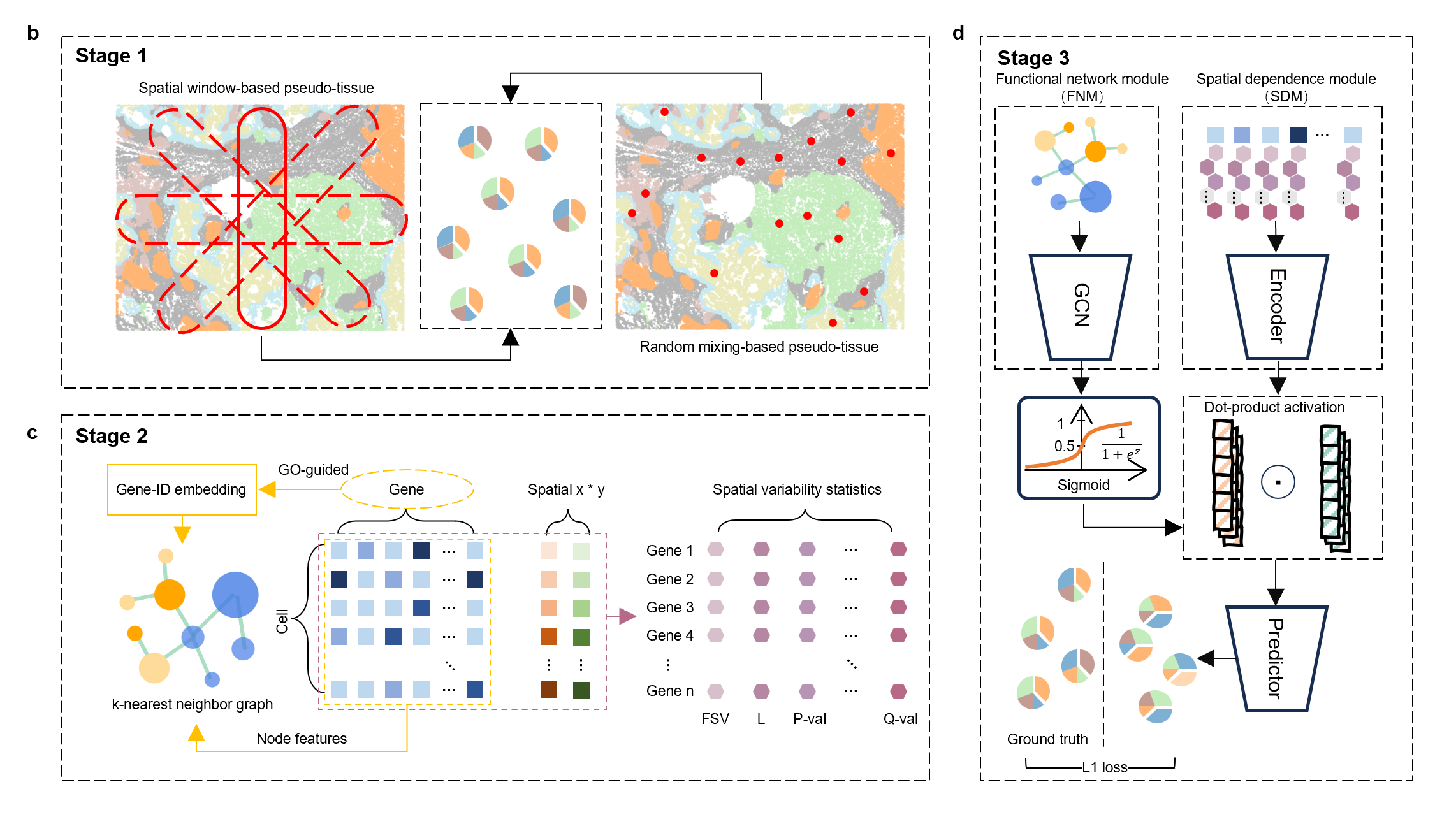
The notebook reads nanostring_cosmx_human_nsclc_reference.h5ad, normalizes counts, splits batches into training and testing samples, removes rare niches from the training set, generates spatial sliding-window pseudo-bulk profiles at multiple rotation angles, adds random mixed-cell pseudo-bulk profiles, and writes nsclc_norm.

CODEX example

cd data/CODEX
jupyter lab data_process.ipynb

The notebook reads nor_log1p_codex.h5ad, maps CellCharter clusters to niche labels, splits BALBc samples, generates pseudo-tissue profiles, normalizes them, and writes CODEX_norm.

Train and predict

After pseudo-tissue data and graph files are available, run the model notebooks from their experiment folders.

Human NSCLC model

cd exp/human_nsclc
jupyter lab model_nicheDeconv.ipynb

CODEX model

cd exp/CODEX
jupyter lab model_nicheDeconv.ipynb

Each notebook loads normalized pseudo-tissue data, appends spatial variability features, builds the GCN gene graph tensors, registers the graph with nicheDeconv, trains with early stopping, computes CCC, RMSE, and Pearson correlation, and saves predictions.

model = nicheDeconv(num_epochs=200, batch_size=50, learning_rate=0.0001)
model.register_graph(edge_index, edge_weight, len(gcn_gene_names))
pred_loss, best_model_weights = model.train(source_data, target_data, valid_data, patience=10, tissue_name="human_nsclc")
target_preds, ground_truth = model.prediction(model.test_target_loader)
CCC, RMSE, Corr = compute_metrics(target_preds, ground_truth)

Expected outputs

Successful runs write model checkpoints and CSV files with predicted and true niche proportions.

Dataset	Prediction file	Ground truth file	Checkpoint
Human NSCLC	`res/human_nsclc/nicheDeconv.csv`	`res/human_nsclc/real_ncslc.csv`	`save_models/human_nsclc/best_model.pt`
CODEX	`res/CODEX/nicheDeconv.csv`	`res/CODEX/real_CODEX.csv`	`save_models/CODEX/best_model.pt`

Troubleshooting

Imports fail in Jupyter

Start Jupyter Lab from the repository root, or add the repository root to PYTHONPATH before running notebooks.

Training is slow or CUDA is unavailable

The example model code uses CUDA tensors. Use a CUDA-enabled environment for direct reproduction, or adapt the model code to select CPU tensors when no GPU is available.

Required input files are missing

Download the full data archive from Zenodo and place dataset-specific files in the corresponding data/human_nsclc/ or data/CODEX/ folder before running the notebooks.